1951 年，剑桥大学的计算机停了六个月。生理学家安德鲁·赫胥黎正等着用它，求解他和同事艾伦·霍奇金刚写下的一组方程。

这组方程描述一种鱿鱼神经细胞怎样发放电脉冲，也就是动作电位。神经细胞靠这类电脉冲交流，大脑从感知到智力的活动都建立在此之上。要知道方程能不能用，只能先把它们解出来，再拿去和实测数据对比。

计算机用不了，赫胥黎只能改用手摇机械计算器。这个过程花了三个多星期。

模型的基本结构，来自当时对细胞的已知事实。他们把细胞膜看成一个电路。可有一块只是有根据的猜测：为了让曲线对上已经测到的数据，他们发现必须把某个变量提高到四次方，也就是自己乘自己三次。当时他们并不知道为什么非这样不可，只知道不这样做，模型对观测数据的预测就会变差。

他们还是谨慎地提出了一个假说。控制细胞膜上某些通道如何打开的那个变量，之所以要用四次方，可能是因为膜里要有多个带电粒子先各就各位，通道才会打开。

几十年后，另一支团队解析了一种相关钾离子通道蛋白的结构，发现它确实由四块相同的部分围着中央孔隙排列。那时霍奇金和赫胥黎已经因 1963 年的诺贝尔生理学或医学奖而为人所知。这套模型在 1951 年是按当时的数据拟合的，当时就已经能比较准确地预测冲动传播得有多快。它后来还帮助人们预测了钾离子通道本身的结构，而模型当初并没有拿这部分结构来拟合。

作者写道，今天的 AI 系统，按说可以在一个下午里找出类似霍奇金与赫胥黎那样的方程，拟合实验数据时也许还会更贴。可这个故事的要点在于：只知道四次方能把活干完，还不够。更要紧的是知道，更简单的版本做不到。一个只把模型交到你手上的 AI 系统，可能给了你一个答案，却没有给你理解。用一个模型复现数据是不够的，因为能做到这一点的模型可以有很多个。真正要紧的，是能够对真实世界里的系统本身作出断言，最好还能对其他相似的系统作出断言。要做到这一点，你需要知道这个模型和其他行得通的模型共享哪些特征，又和那些行不通的模型差在哪里。数学家理查德·汉明在 1962 年写道：The purpose of computing is insight, not numbers.

这是 Jakob Macke、Daniel Gedon 和 Stefan Wahl 在 Anthropic 科学博客上的客座文章。三位作者是图宾根大学和 ELLIS Institute Tübingen 的研究者，也是 Anthropic AI for Science 项目的资助对象，他们在神经科学及其他领域开发用于构建科学模型的 AI 工具。文章由 Anthropic 官方账号在 2026 年 11 月 6 日转发，文中的判断来自这三位作者，编辑审阅由 Xander Balwit、Tom Chivers 和 Siddharth Mishra-Sharma 协助。

建模常见的三步：写出形状、用数据收紧、再解释含义

七十多年过去了，霍奇金-赫胥黎模型 仍是描述神经元电活动的标准说法。同类方程只要换一套常数，就能描述从鱿鱼到人类的神经细胞，尽管这两支演化谱系分开已经超过五亿年。

比它活得久更重要的，是它把建模这件事拆开了。作者认为，霍奇金和赫胥黎的做法可以分成三步，大多数科学建模都有某种对应版本。

第一步是构建模型：决定模型由什么组成，方程取什么形状。对他们来说，就是电路里的膜和通道，以及把那个变量提到四次方这样的方程形式。

第二步是约束模型：调节可调参数，让它贴上真实测量。比如在不同电压下，通道打开有多频繁。

第三步是解释模型：追问模型对真实系统说了什么。比如四次方是否意味着通道有四个活动部件。

科学家通常会反复走这三步。数字对不上测量，或者解释说不通，就退回去改。这三步从前都由人来做，现在 AI 系统越来越多地参与每一步。作者认为，机器目前进展最大的，可以说是约束模型，所以他们先从这里讲起。

一笔 120 美元的账单，对得上很多种点单

霍奇金和赫胥黎当年靠眼睛和直觉来收紧模型，最后得到的是一组数字。这组数字说明模型可以对上数据，却没有告诉他们：别的数字是否也能一样好，甚至更好。

文章用一顿合计 120 美元的聚餐账单来类比。你只知道总账，不知道谁点了什么。谁都点了中等价位的汉堡，或者一个人点了牛排和龙虾、其他人只喝汤，都有可能加总成这个数。神经细胞模型也是这样：不同的通道参数组合，可以产生几乎相同的电活动。只展示一组拟合得好的数字，等于把其他说得通的参数设定都藏起来了，而那些组合可能导向不同的预测。作者认为，几乎任何被建模的现象都是如此，很多组不同的参数都能同样好地解释观测到的数据。

原文图 1 是嵌在网页里的交互说明，地址是 https://assets.claude.ai/brand/artifacts/research/teaching_ai.html 。图里有三部分：神经细胞的一次测量；钾通道和钠通道各种组合有多可能解释这次测量，颜色越深表示拟合越好，蓝点可以拖动；以及三组设定下的模拟，和灰色的测量曲线放在一起对比，有的对得上，有的对不上。本站无法把这个可拖动的控件保存成静态附件，读者可以打开原页自己试。

统计上的办法叫贝叶斯推断。它给出每一组还算说得通的数字，形成一个概率分布，既考虑这些数字和数据的拟合程度，也考虑你对参数已有的先验认识。这个分布像一条曲线，拟合最好的在峰顶，较弱的在边缘。

对复杂模型来说，这种方法通常并不实用，因为它要计算：在每一组可能的数字下，你测到的结果有多可能出现。霍奇金和赫胥黎的模型规模还做得到；再复杂一些，计算上就不可能了。比如成千上万个离子通道各自随机开合，你就得穷尽每一种组合。回到那张账单：回答“如果 A 点了汉堡、B 点了牛排，账单会是多少”并不难；反过来指出哪些组合能加总成最终账单，人一多、菜单一长，就要难得多。

另一种办法叫基于模拟的推断，简称 SBI。它靠大量计算来处理这种反向工程。你随机挑选参数，运行模型，记下输出，然后一遍遍重复。对类似霍奇金-赫胥黎这样的模型，大约要跑 10 万次；更大、更复杂的模型则要数百万次。再用这些结果训练一个神经网络：给它一个输出，它就能返回可能产生这个输出的参数范围。

SBI 只要求你能把模型正向跑起来：输入一组参数，得到你预期会看到的那类数据。这样“参数进去、数据出来”的模型叫做模拟器，也就是 simulation-based inference 这个名字的来历。你不必再用公式去计算测量结果有多可能出现，而那一步正是标准贝叶斯推断常常无法实施的原因。今天的模拟器通常是计算机程序，但并非必须如此。赫胥黎当年用手摇计算器一步步算方程，其实也是在运行一个模拟器。许多模拟器正向容易、反向几乎不可能。有些甚至写不成整齐的方程，假设就写在它们遵循的规则里，但它们仍然是模型。从神经元网络到星系碰撞，对许多复杂现象来说，模拟器常常是我们仅有的模型种类。SBI 让这类模型也能被数据约束。

跑完这些模拟代价很高，有时要花上几周。一旦完成，训练好的网络可以在几秒内对新数据做推断，不必再跑新的模拟。这种速度改变了能做的事。两颗中子星碰撞时，SBI 可以大致判断碰撞发生在天空的哪个位置，快到足以在信号还能被探测到时把望远镜指过去。同一思路也已经用在宇宙学、结构生物学、地球物理学和许多其他领域。

SBI 也被用到了神经细胞模型，包括霍奇金-赫胥黎模型本身。因为它返回的是一个分布，而不是单次拟合，研究者可以看到哪些参数被数据约束得很紧，哪里存在不止一种说得通的解释，以及最需要更多数据、也就是下一场实验的地方在哪。

模型这一层，同样不该只交出一个答案

要约束一个模型，先得有一个模型可约束。霍奇金-赫胥黎模型的方程并不是从第一性原理推出来的。那个变量的四次方，是从科学家的生物学直觉里长出来的，也来自他们发现更简单的版本效果不够好。

在科学史的大部分时间里，模型都是这样建出来的：研究者凭经验和假设写下候选，再检验、修改、重来。问题在于，可能的模型空间本质上是无穷的。一个科学家凭经验只提出少数几个模型，很可能会漏掉那些同样能解释观测数据的模型。

AI 系统现在可以帮忙，甚至接手这一步。给定一些数据和一段对系统的自然语言描述，基于大语言模型的智能体会为候选模型或一组候选模型写代码，然后运行模型、约束参数、把输出和真实世界的数据对比，再修订它，也许是改一个方程的形式。这个循环一直重复，直到模型足够准确地复现数据。过去两年里已经出现了好几套这样的系统，作者举例提到 Romera-Paredes 等人 2024 年、Shojaee 等人 2025 年、Ma 等人 2024 年、Novikov 等人 2025 年、Xia 等人 2026 年，以及 Ziaei Bideh 与 Gryak 2026 年的工作。细节各不相同，但都用大语言模型来设计模型本身。直到最近，这一步仍被认为只有人类能做。

可是，模型能复现数据，并不等于它提供了洞察。就像那张聚餐账单，或霍奇金-赫胥黎模型里的参数，同一模型内部许多不同的参数组合可以给出相同输出。再往上一层，对模型本身也成立：许多方程形状不同的模型，可以同样好地解释同一批数据。把一个智能体在同一批数据上跑两次，它可能返回两个不同、却同样好的模型。一个只交出其中之一的智能体，等于把其余的都藏起来了，就像只展示一组最佳拟合数字。

所以，构建模型最好也用约束模型的办法：去要全部那些有可能解释数据的模型。他们指向 Wahl 等人 2026 年、Mishra-Sharma 2026 年和 Murphy 2026 年的讨论。AI 系统提出许多候选，再按数据对每个候选的支持程度加权。那些必须非常灵活才能拟合上的模型，得到的分量会低于那些自然就能拟合的模型。弱的候选被淘汰，系统再对更强的那些提出新的变体。

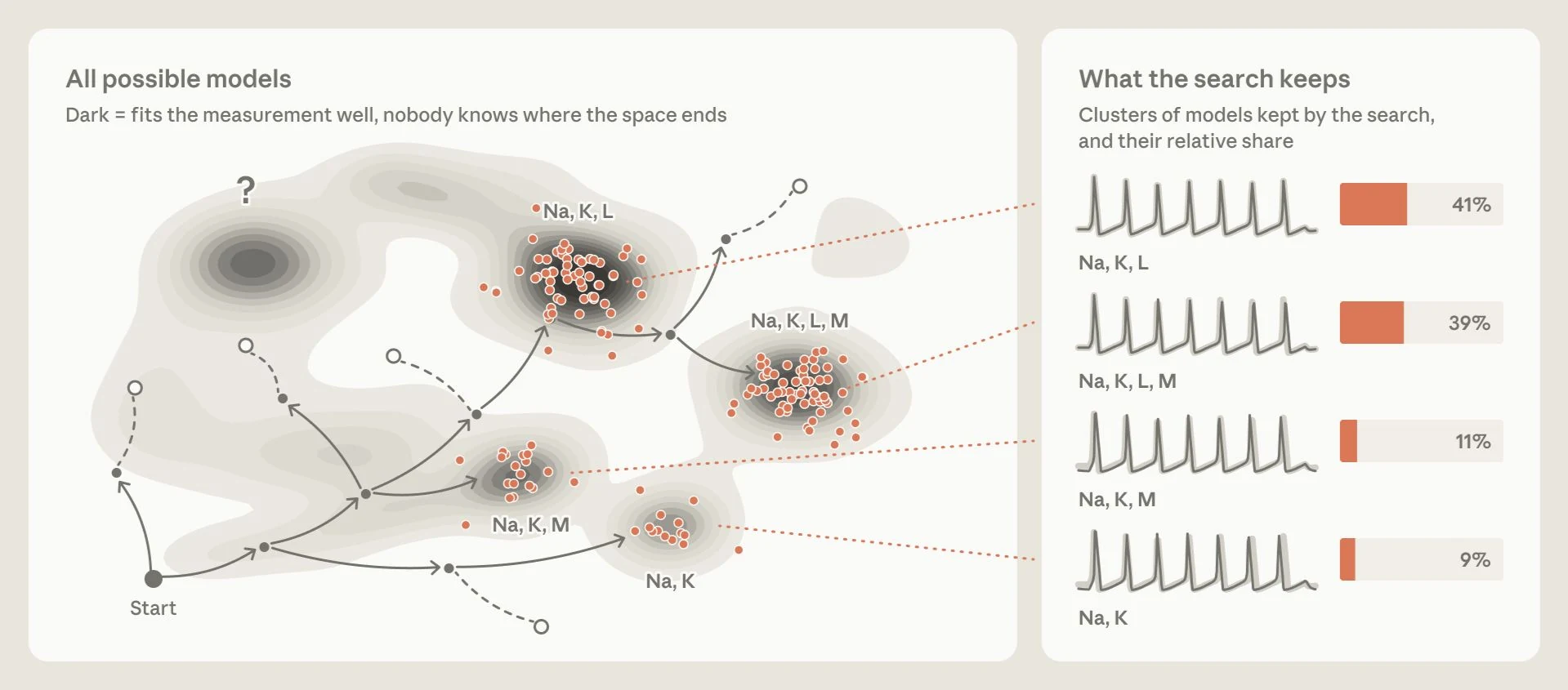
图 2 把这个搜索画了出来。左侧每个点都是霍奇金-赫胥黎模型的一种可能变体，背景越暗表示模型越可能；搜索从起点向外分支，并在若干区域聚成簇。右侧是每个簇里由 AI 系统构建的模型模拟，以及各簇占全部模型的份额：41%、39%、11% 和 9%。作者写道，他们会同时保留更可能和不太可能的模型，因为所有模型都可能带来洞察。

这样，智能体就能提供一组说得通的模型，而不是单个最佳拟合。这个分布能告诉你单个模型说不出来的事。如果所有存活下来的模型都共享某个特征，数据很可能支持它。如果它们意见不一，说明证据还薄，也会把研究者指向下一场实验。

作者提醒不要走得太远。到目前为止，这些系统大多还在重新发现科学家已经知道的模型。它们能否处理没有已知答案的问题，证据仍然很少。不过，更新的大语言模型在研究任务上的表现已经好于更早的模型，作者预计这些系统还会继续改进。

解释是三步里最难交给 AI 的一步

模型被写出来、又被数据收紧之后，还得解释：它到底对正在研究的真实系统说了什么？霍奇金和赫胥黎的“四个粒子”假说，来自一个推论：如果通道打开前必须先发生四件分开的事，方程里就会出现四次方。于是他们推测，膜里面可能就是这样。后来看，这个判断大体是对的。

这个解释之所以站得住，是因为他们排除了别的可能。如果更简单的模型也能一样好用，就没有理由认为通道有好几个活动部件。是替代方案的失败，才让他们能提出这个断言。确切数字当时也有不确定：他们注意到需要三次方或四次方，最后选定了四。他们写道，更高的次幂也许还能拟合得稍好一点，但那点改进不值得再增加复杂程度。

这套方程还让他们推出了另外几层含义。比如，它解释了为什么神经细胞存在一个电压阈值，低于它不会发放、高于它才会发放，以及为什么神经脉冲都有相同的形状。它还预言：如果电流上升得足够慢，细胞将永远不会发放。科学哲学家把一种理论称为“可理解的”，如果它让你不必运行模型，就能推出它的后果。这个标准适用于变量只有少数几个的模型，霍奇金-赫胥黎模型就是如此。对一个可能有数千个变量的更大模型，对应的标准也许是：我们能不能把它收成几个关键的机制想法，而这些想法又足以把它重建出来。模型越大，这一点就越难。

在作者看来，三步里最难交给 AI 的，就是解释。目标更难钉死：模型拟合数据好不好，可以测量；它有没有带来对系统更好的理解，却量不出来。也不清楚该怎样让 AI 系统把“理解”当成优化目标。一种提议是看它能否预测：当你扰动这个系统时，系统会怎样变化。另一种办法是先绕开这个问题，改问智能体的输出能不能帮助人类科学家更好地理解问题。一个例子是用于设计量子实验的 AI 系统。它不被训练成只给出一套装置，而是写出一个短程序，生成一整族相关实验的装置。物理学家就可以直接从程序里读出底层设计原则，而不必从某一套实验装置反向还原。

这两种路径里，能看到一整组合适的模型，而不是单个拟合得最好的模型，对解释都至关重要。单个模型无法告诉你，它的哪些部分真正被数据约束住了，于是很容易把意义读进那些其实没被钉住的部分。在霍奇金-赫胥黎模型里，关于四个粒子的假说，只有在你知道更低次幂效果不够好时才说得通。一组模型也会让预测更稳妥。比如你问这些模型：如果把细胞膜上的钠通道全部堵住，或只堵住一部分，会发生什么。如果所有拟合数据的模型都给出同一个答案，就像全部通道都被堵住时你预期会看到的那样，这个答案就可以比较有把握。如果它们意见不一，比如只堵住一部分通道时就可能出现这种情况，这本身就能给下一场实验提供想法。

从一只神经细胞，到一只果蝇的整个大脑

包括霍奇金-赫胥黎模型在内，大多数著名模型都很紧凑：只有少量变量和方程，小到人类科学家可以写下来、也可以推理。这并非巧合。它们必须小，因为人得亲自构建、约束和解释它们。小，也正是它们可被理解的原因。可当 AI 接手更多工作时，这个体量上限会开始松开。我们可以开始为那些手工根本写不下来的复杂系统建模，即便再也无法只靠读方程来理解它们。

大脑是一个很直接的应用场景。霍奇金-赫胥黎方程描述的是单个神经细胞。果蝇的大脑有超过 10 万个神经元，人脑则有数百亿个。行为与思维，来自这些神经元之间的相互作用。对果蝇，现在有了前几代科学家不可能拥有的东西：一张完整的大脑接线示意图，标出每一个神经元，以及它们怎样彼此连接。作者提到的相关工作包括 Dorkenwald 等人、Schlegel 等人，以及 Azevedo 等人 2024 年的研究。研究者已经开始在这张图上建立大规模模型，其中一套可以预测果蝇视觉系统中神经元的活动。于是一些从前没法认真提出的问题出现了：整个大脑怎样把接线变成行为？一种动物的行为有多少能只从接线预测出来？哪些连接才真正要紧？

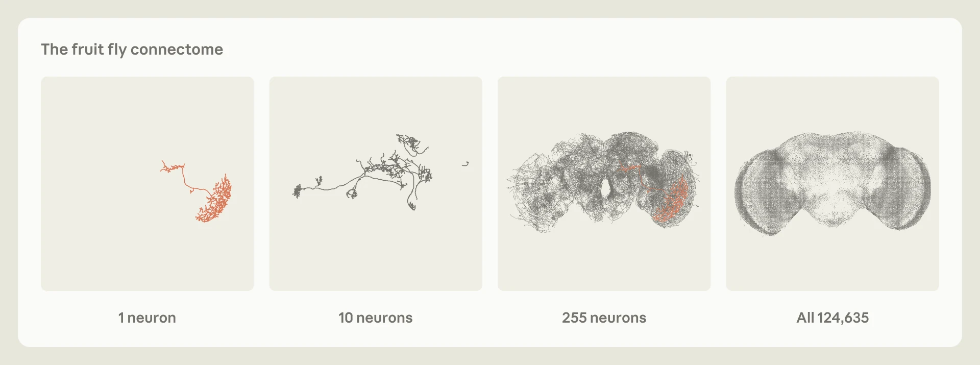
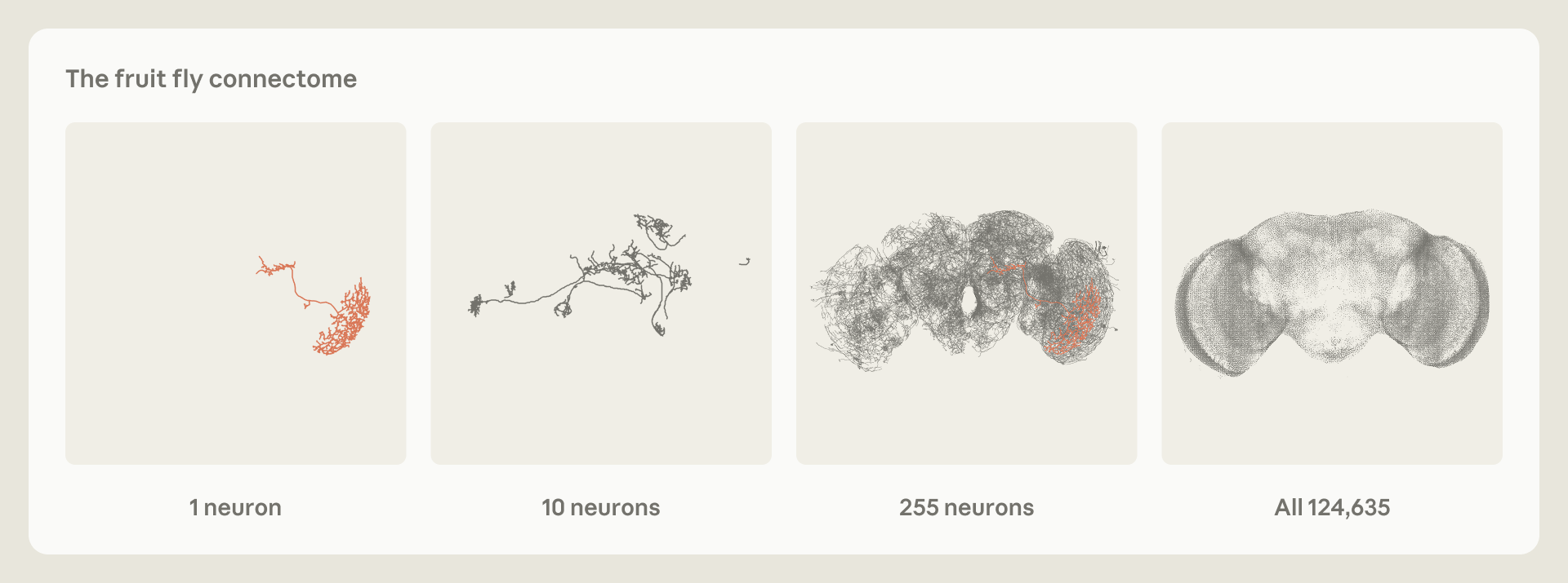
图 3 按果蝇中枢神经系统的完整接线示意图绘制，依次显示 1 个、10 个、255 个神经元，以及全部 124,635 个细胞。第 1 幅和第 3 幅里，有一个神经元用橙色标出。图像来自雄性中枢神经系统连接组，由 HHMI Janelia、剑桥大学、MRC LMB 和 Google Research 提供，采用 CC BY 4.0 许可。

这并不只发生在神经科学里。气候科学家已经这样工作：他们建立许多巨型数值模拟，各自基于略有不同的假设，再把预测报告成所有这些模拟之间的分布。大型强子对撞机上的粒子物理学家也有类似思路：寻找新粒子时，他们不会只宣布某个特定理论成立或不成立，而会画出一张地图，标出该理论的哪些版本已被数据排除，哪些仍然开放。

霍奇金和赫胥黎当年那些费力的工作，构建模型、用眼睛拟合每条曲线、试过那些拟合不上的次幂，以及赫胥黎花三个星期手摇计算器，并不是人们想回到的日常。可这些功夫没有白费。一个模型提供的许多洞察，来自创造它的过程。他们理解模型在说什么，是因为模型是自己建出来的，也知道哪些路没走通。正是这种理解，让他们形成了对门控变量的解释，而这是后来为他们赢来诺贝尔奖的发现的一部分。

作者认为，AI 系统现在按说可以在一个下午里完成其中许多工作。可它如果要提供理解，就得交出这两位科学家缓慢工作所产生的东西：不只是那个拟合上的模型，还要说明哪些部分被数据钉住了，哪些仍然开放，沿途哪些替代方案失败了，过程中又冒出了哪些新的谜题。科学模型可以提供一个答案，但给出洞察的，是构造它的过程。

下次看到一个拟合得很好的科学模型，无论它出自人手还是 AI，都可以先问几句。还有哪些模型同样解释得通？哪些部分真的被数据钉住了，哪些只是看起来像那么回事？存活下来的模型在哪些地方意见不一？

作者认为，最有用的下一步实验，往往是那些能一次排除最多剩余模型的实验，哪怕它们不一定是研究者自己最感兴趣的那几个。他们也写明了眼下的边界：这些系统目前大多还在重新发现科学家已经知道的模型；它们能否处理没有已知答案的问题，证据仍然很少。一个下午交出来的漂亮拟合，可以当作候选解释，还不能单独当成对真实系统的理解。

原文媒体未在改写中展示：原文图 1 是嵌在文章中的交互式 HTML 说明（https://assets.claude.ai/brand/artifacts/research/teaching_ai.html），可以拖动蓝点，查看不同钠通道和钾通道组合下的模拟是否拟合测量曲线。本站无法把该控件保存为可拖动的静态附件；图注与机制已在正文说明，读者可打开原页或上述链接自行操作。

Teaching AI to build scientific models

Published Nov 6, 2026 · Team: Science · Topics: Discovery, Research programs, Life sciences

AI for Science grantees Jakob Macke, Daniel Gedon, and Stefan Wahl are researchers at the ELLIS Institute Tübingen and the University of Tübingen, where they build AI tools for developing scientific models in neuroscience and beyond. In this guest post, they discuss how AI is starting to change scientific modeling.

In 1951, Cambridge University’s computer went out of action for six months. This was inconvenient for physiologist Andrew Huxley, who, alongside his colleague Alan Hodgkin, had just built a set of equations to describe how a particular squid nerve cell fired. The scientists wanted to understand the “action potential” of these nerve cells: the electrical pulses they use to communicate, which underlie everything brains do, from perception to intelligence. The only way to find out whether the equations worked was to solve them and compare the solutions to data.

Huxley had hoped to use the newfangled computer to solve the equations. Instead, he was forced to solve them using a hand-cranked mechanical calculator. It took him over three weeks.

The basic structure of their model was dictated by known facts about the cell. Hodgkin and Huxley modeled its membrane as an electrical circuit. One part of the model, however, was just an educated guess. In order to make the curve fit the data they had measured, they found that they had to raise one variable to the fourth power—that is, to multiply it by itself three times. At the time, they did not know why. They just knew that otherwise the model didn’t predict the observed data as well.

They did offer a hypothesis, however. They cautiously suggested that the variable in question, which governed how particular gates in the cell membrane opened, might require the fourth power because multiple charged particles in the membrane had to move into place before the gate would open.

Decades later, long after both Hodgkin and Huxley had won the Nobel Prize in Physiology or Medicine in 1963, another team found the structure of a related potassium channel protein. And they discovered that, yes, it had four identical pieces arranged around a central pore. The model was fit to the data in 1951. Even then, it predicted how fast the impulse travels relatively accurately. More than that, it turned out to have helped predict the structure of potassium ion channels themselves, which it had never been fit to.

Today, an AI system could plausibly find an equation like Hodgkin and Huxley’s in an afternoon, and perhaps it would fit the experimental data even more closely. But the point of the story is that simply knowing the fourth power did the job was not enough; what mattered was knowing that a simpler version of the model did not work. An AI system that merely hands you the model might give you an answer, but it does not give you understanding. Reproducing the data with a model is insufficient, because any number of models could do the same. What matters is being able to make claims about the real-world system itself, and ideally about other, similar systems. To do so, you need to know which features the model shares with other models that work, and which set it apart from models that don’t. As the mathematician Richard Hamming wrote in 1962, “The purpose of computing is insight, not numbers.”

A three-step program

More than 70 years on, the Hodgkin-Huxley model remains the standard description of electrical activity in neurons. The same kinds of equations, with different constants, describe nerve cells across the animal kingdom, from squids to humans, even though our evolutionary lineages separated more than half a billion years ago.

Even more important than its longevity, however, is what the Hodgkin-Huxley model tells us about how models work. Hodgkin and Huxley’s approach can be broken down into three steps, and most scientific modeling involves some version of them.

• The first is building the model. This means deciding what the model is made of and what shape its equations take. In Hodgkin and Huxley’s case, that meant the parts of the electrical circuit—the membrane and the gates—and the form of the equations, such as raising the underlying variable to the fourth power.
• The second is constraining the model—tuning its adjustable parameters to fit real measurements. For Hodgkin and Huxley, that included settings like how often the gates open under different voltages.
• The third is interpreting the model—asking what the model says about the real system, such as suggesting that the fourth power meant the gate had four moving parts.

In practice, scientists go through these steps repeatedly. If the numbers fail to fit the measurements, or if the interpretation makes no sense, they go back and revise.

All three steps were once done by people, but AI systems are increasingly involved in each of them. Machines have arguably made the most progress in constraining models, so we’ll start there.

Splitting the bill, or how to constrain models

When Hodgkin and Huxley constrained their model by eye and intuition, they ended up with a single set of numbers. This told them that the model could match the data. It didn’t tell them whether other numbers would have worked just as well or even better.

Imagine you know that a group dinner added up to $120, but not who ordered what. Many different combinations of orders could have added up to that amount—perhaps everyone ordered a mid-priced burger, or perhaps one person had steak and lobster while everyone else had soup. Models of nerve cells work on the same principle: different combinations of gate parameters can produce near-identical electrical activity. Simply showing one combination that fits well hides all the other plausible parameter settings, and other combinations might have led to different predictions. This is true of almost any phenomenon being modeled. Many different sets of parameters can explain the observed data equally well.

Figure 1 is an interactive illustration embedded from https://assets.claude.ai/brand/artifacts/research/teaching_ai.html

Figure 1. An illustration of constraining the Hodgkin-Huxley model. (1) A measurement from a nerve cell. (2) How likely the measurement is for each combination of potassium and sodium channel settings. Darker means a better fit. The blue dot is interactive. (3) Simulations of the model at three settings, compared to the measurement (gray). Some fit well, while others do not.

The solution is a statistical method called Bayesian inference. It gives you every set of numbers that works reasonably well, as a probability distribution that takes into account their fit to the data and your prior knowledge about the parameters. The distribution takes the shape of a curve, with the best fits at the peak and the weaker ones at the fringes.

But this method has usually been impractical for complex models, because it involves calculating how likely your measurements would be under every possible set of numbers. In Hodgkin and Huxley’s model, that would still be feasible, but for anything more complicated, it would be computationally impossible. For example, if each of the thousands of ion channels opens and closes at random, you would have to work out every combination. Returning to our restaurant bill analogy: it would be easy to answer, “If person A had the burger and person B had the steak, what would the bill come to?” but much harder to show which combinations could have led to the final bill, especially as the number of people and menu options grows.

A different approach called simulation-based inference (SBI) overcomes this reverse-engineering problem with sheer computation. You pick random parameters, run the model, and record the output. You do it again and again— perhaps 100,000 times for a model like Hodgkin-Huxley, and millions of times for larger, more complex ones. Then you train a neural network on the results so that, given an output, it can return the range of parameters that could have produced it.

All SBI requires is that you can run the model: put in a set of parameters and get back the kind of data you would expect to see. A model you can run like this—parameters in, data out—is called a simulator, hence the name “simulation-based inference.” You never need to use a formula to calculate how likely your measurements are, which is the step that makes standard Bayesian inference often impractical. These days a simulator is usually a computer program, but it doesn’t have to be: Huxley, cranking through the equations by hand, was running one. Many simulators are easy to run forward but impossible to reverse. Some can’t even be written out as a tidy equation—their assumptions are built into the rules they follow—but they are models nonetheless. For many complex phenomena, from networks of neurons to colliding galaxies, simulators are often the only kind of model we have. SBI lets us constrain those models with data.

Running all those simulations is expensive and can take weeks. But once it is done, a trained network can perform inference on new data in seconds, without requiring further simulations. That speed has changed what’s possible. When two neutron stars collide, SBI can work out roughly where in the sky the collision happened, fast enough to point telescopes at it while the signal is still detectable. The same approach has been successfully applied to problems in cosmology, structural biology, geophysics, and many other domains.

And SBI has been applied to nerve cell models, including the Hodgkin-Huxley model. Because it returns a distribution rather than a single fit, we can see which parameters are well constrained by the data, where more than one explanation is plausible, and where more data—and thus another experiment—is most needed.

The bill, one level up, or how to build models

Before you can constrain a model, you need a model to constrain. The equations of the Hodgkin-Huxley model were not derived from first principles. Instead, the fourth power of the underlying variable emerged empirically from the scientists’ biological insight, and from finding that simpler versions didn’t work as well.

For most of the history of science, this is how models have been built. Scientists used their expertise and assumptions to write down a candidate model. Then they tested it, revised it, and tried again. The problem is that the space of possible models is essentially infinite, and a scientist proposing a handful of models from experience will very likely miss models that could have explained the observational data equally well.

AI systems can now help with, or even take over, this step. Given some data and a natural-language description of a system, an LLM-based agent writes code for a candidate model or a set of candidate models. Then it runs the model, constrains its parameters, compares the output to real-world data, and revises it, perhaps by modifying the form of an equation. This loop repeats until the model replicates the data accurately enough. Several such systems have appeared in the past two years.1 The details vary, but all use an LLM to design the model itself. Until recently, this was thought to be something only humans could do.

But the fact that a model replicates data doesn’t mean that it provides insight. As with the restaurant bill, or the Hodgkin-Huxley parameters, many different combinations of parameters within a single model can provide the same output. The same is true one level up, for the model itself: many different models, with differently shaped equations, can explain the same data equally well. Run an agent twice on the same data, and it might return two different, and equally good, models. An agent that returns only one of them is hiding the rest, just as a single best-fit set of numbers does.

So it is better to treat building a model the same way we treat constraining one: you ask for the whole range of models that could plausibly explain the data.2 The AI system proposes many candidates. Each is then weighted by how much it is supported by the data, and the ones that need a lot of flexibility to fit are given less credit than those that fit naturally. The weak candidates drop out, and the AI system proposes new variations on the stronger ones.

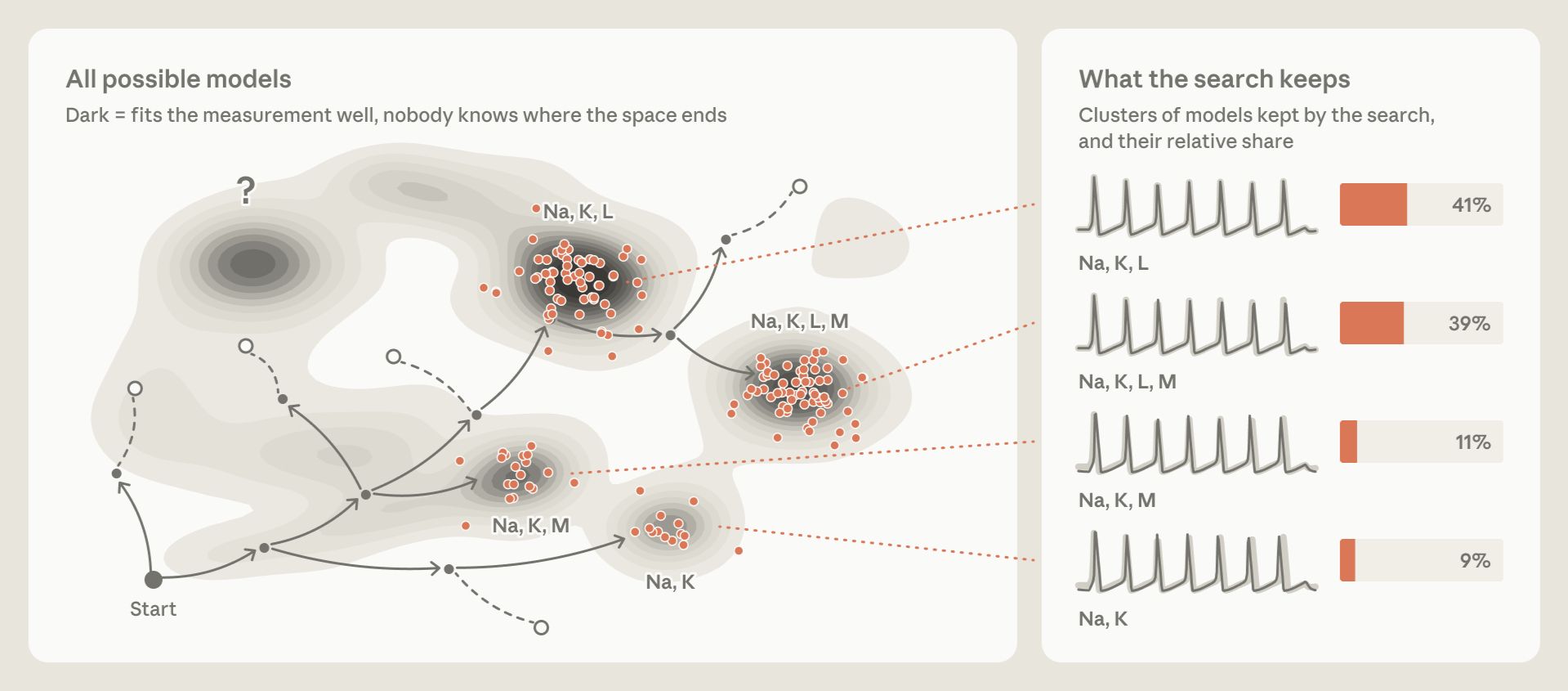
AI agents can thus provide a distribution of plausible models, rather than a single best fit, and that distribution tells you things a single model can’t. If every surviving model shares a feature, the data likely favors it. If the survivors disagree, that shows where the evidence is thin, and points researchers in the direction of the next experiment.

We shouldn’t get too far ahead of ourselves. So far, these systems have mostly been tested on rediscovering models that scientists already know. Evidence that they work on problems with no known answer is sparse. Still, newer LLMs perform better at research tasks than older ones, and we expect these systems to keep improving.

Lost in translation, or how to interpret models

Once a model has been built and constrained, it still has to be interpreted. What does it tell us about the real system being studied? Hodgkin and Huxley’s four-particle hypothesis came about because equations involving the fourth power are what you would expect if four separate things all had to happen before a gate could open. So they suggested that this might be what was happening inside the membrane. As we saw above, they turned out to be largely right.

That interpretation only carried weight because of what they had ruled out. If a simpler model had worked just as well, there would have been no reason to think the gate had several moving parts. It was the failure of the alternatives that allowed them to make that claim. There was some uncertainty about the exact number: Hodgkin and Huxley noted that a third or fourth power was needed and settled on four. They wrote that higher powers might even have fit slightly better, but that the potential “improvement was not considered to be worth the additional complication.”

The equations also let Hodgkin and Huxley reason out several other implications. For instance, the equations explained why nerve cells have a voltage threshold below which they don’t fire and above which they do, and why nerve pulses all have the same shape. They also predicted that a current rising slowly enough would never make the cell fire. Philosophers of science call a theory “intelligible” if it lets you work out its consequences without having to run it. That test works for a model with a handful of variables, like Hodgkin-Huxley. For a larger model with perhaps thousands of variables, the equivalent might be whether we can boil it down to a few crucial mechanistic ideas that are enough to rebuild it. The larger the model, the harder that becomes.

Of the three steps, interpretation is the hardest to hand over to AI. The goal is harder to pin down: we can measure how well a model fits the data, but not whether it leads to a better understanding of the system, and it’s not clear how to tell an AI system to make “understanding” its objective. One proposal is to judge an AI system’s understanding by seeing how well it predicts what a system does when you disturb that system. Another is to sidestep the question altogether, and instead ask whether the agent’s outputs help human scientists better understand the problem. One example is an AI system for designing quantum experiments. Rather than providing a single setup, it was trained to write a short program that generates the setups for a whole family of related experiments. A physicist can then read the underlying design principle straight off the program instead of reverse-engineering it from one experimental setup.

In both approaches, having access to a full distribution of suitable models, rather than a single best-fitting one, is crucial for interpretation. A single model cannot tell us which of its parts are actually constrained by the data, so it’s easy to read meaning into parts that are not. In Hodgkin-Huxley, as we’ve seen, the hypothesis about four particles only makes sense if you know that lower powers don’t work as well. A range of models also makes predictions more robust. Say you ask your models what happens when you disturb a system—for instance, by blocking all, or only some, of the sodium gates on the cell membrane. If all the models that fit the data return the same answer, as you would expect when every gate is blocked, then you can be fairly confident in it. If they disagree, as they might when only some gates are blocked, that can provide ideas for the next experiment.

Cells and scales

Most famous models, including Hodgkin-Huxley, are compact. They consist of a handful of variables and equations, small enough for a human scientist to write down and reason about. That’s no coincidence: they needed to be compact, because people had to build, constrain, and interpret them. Their smallness is also what made them intelligible. But as AI takes over more of the work, the size limit will start to lift. We can begin to model systems that are far too complex to write down by hand, even if we can no longer understand them just by reading the equations.

Brains are an obvious use case. The Hodgkin-Huxley equations describe a single nerve cell. But a fruit fly’s brain contains more than 100,000, and a human brain tens of billions. And it is the interplay between those neurons that gives rise to behavior and thought. For the fruit fly, we now have something that was impossible for previous generations of scientists: a complete wiring diagram of its brain, showing every neuron and how it connects to the others.3 Researchers have started building large-scale models on top of it, including one that predicts the activity of neurons across the fly’s visual system. That opens up questions nobody could sensibly ask before. How does a whole brain turn its wiring into behavior? How much of an animal’s behavior can be predicted from its wiring alone? And which connections actually matter?

This isn’t unique to neuroscience. Climate scientists already work like this: they build many gigantic numerical simulations, each based on slightly different assumptions, and report their projections as the spread across all of them. Particle physicists at the Large Hadron Collider work in a similar spirit: when they look for a new particle, they don’t just declare whether a particular theory worked or not; they produce a map of which versions of the theory are ruled out by the data and which remain open.

The painstaking work Hodgkin and Huxley did—building the model, fitting each curve by eye, trying the powers that didn’t fit, and, in Huxley’s case, spending three weeks hand-cranking the mechanical calculator—is not something we want to go back to. But it was not wasted. Much of the insight that a model provides comes from the process of creating it; Hodgkin and Huxley understood what the model was telling them because they had built it themselves, and they knew what hadn’t worked. This understanding let them formulate their interpretation of gating variables—part of the discovery that ultimately earned them the Nobel Prize.

An AI system could now plausibly do much of the same work in an afternoon. But to offer understanding, it needs to deliver what the two scientists’ slow work produced: not just the model that fits, but an account of which parts are pinned down by the data, which are still open, which alternatives failed along the way, and what new puzzles were uncovered in the process. A scientific model may provide an answer, but it is the process of constructing it that provides the insight.

Footnotes

1. See Romera-Paredes et al., 2024; Shojaee et al., 2025; Ma et al., 2024; Novikov et al., 2025; Xia et al., 2026; and Ziaei Bideh and Gryak, 2026, for example.

2. See Wahl et al., 2026; Mishra-Sharma, 2026; and Murphy, 2026.

3. See Dorkenwald et al., 2024; Schlegel et al., 2024; and Azevedo et al., 2024.

Contributors

Jakob Macke, Daniel Gedon, and Stefan Wahl

Acknowledgements

We thank Xander Balwit, Tom Chivers, and Siddharth Mishra-Sharma for review and editorial guidance.

The male CNS connectome figure is rendered from the male CNS connectome (HHMI Janelia, University of Cambridge, MRC LMB, and Google Research), CC BY 4.0.